Dynamic Time Warping (DTW) in Time Series

Dynamic Time Warping

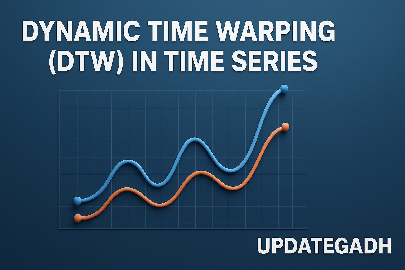
Dynamic Time Warping (DTW) is a powerful algorithm used to measure the similarity between time series that may differ in speed or duration. Unlike standard distance measures such as Euclidean distance, DTW is capable of handling temporal distortions by allowing flexible alignment of sequences. This makes it particularly valuable in fields like speech recognition, bioinformatics, finance, healthcare, and any domain where pattern matching across time series is essential.

Machine Learning Tutorial:-Click Here
Data Science Tutorial:–Click Here
Complete Advance AI topics:-CLICK HERE
DBMS Tutorial:-CLICK HERE

How DTW Works

DTW uses dynamic programming to find the optimal alignment between two time series, even if they progress at different speeds. Unlike Euclidean distance, which compares points strictly one-to-one, DTW can stretch or compress time axes to achieve the best match.

Step 1: Compute the Distance Matrix

The first step is to create a distance matrix between the two sequences. Each entry in this matrix represents the distance (often the absolute or squared difference) between a point in one series and a point in the other.

For example:

• Series A = [1, 2, 3, 4]
• Series B = [1, 1.5, 2.5, 3.5, 4]

The distance matrix allows us to measure pairwise similarities while accounting for possible shifts in timing.

Step 2: Construct the Cumulative Cost Matrix

Next, DTW builds a cumulative cost matrix to identify the least-cost alignment path. The recursive formula is:

C(i, j) = D(i, j) + min(C(i-1, j), C(i, j-1), C(i-1, j-1))

This ensures that the alignment path follows the minimum cumulative distance, allowing flexible matching through diagonal, vertical, or horizontal moves.

Step 3: Trace the Optimal Warping Path

Once the cumulative cost matrix is filled, DTW traces back from the bottom-right corner to the top-left to find the optimal warping path. This path shows how the two series should align, allowing one point in a series to map to multiple points in the other if needed.

Step 4: Compute the DTW Distance

The final DTW distance is the cumulative cost at the bottom-right cell of the matrix. Smaller values indicate higher similarity between the two series.

Key Properties of DTW

To ensure meaningful alignments, DTW follows several important principles:

1. Boundary Condition – The warping path starts at the first elements and ends at the last elements of both sequences.
2. Continuity – The path advances step by step with only adjacent moves (no jumps).
3. Monotonicity – The indices must move forward in time; no backward steps are allowed.
4. Warping Constraint (Windowing) – Limits excessive stretching using techniques like the Sakoe-Chiba band.
5. Slope Constraint – Prevents unrealistic alignment by restricting too many consecutive horizontal or vertical moves.
6. Global Optimality – Guarantees the best alignment by minimizing total cumulative distance.

Applications of DTW

DTW is widely applied in multiple industries and research domains:

• Speech Recognition – Matches spoken words at different speeds for accurate identification.
• Handwriting Recognition – Aligns varying handwriting styles and speeds for text recognition.
• Time Series Analysis & Forecasting – Compares financial data, energy usage, or climate patterns across time.
• Bioinformatics & Genomics – Aligns DNA, RNA, or protein sequences with structural variations.
• Gesture & Motion Recognition – Used in gaming, sports analysis, and healthcare motion tracking.
• Music & Audio Analysis – Syncs different versions of songs or live vs studio recordings.
• Signature Verification – Matches dynamic features like writing speed and pressure for authentication.
• Healthcare – Analyzes ECG and EEG signals to detect abnormalities.

Advantages of DTW

• Flexible Alignment – Works with sequences of varying lengths and speeds.
• Handles Temporal Distortions – Effective even when events occur at different paces.
• Robust to Noisy Data – Tolerates small distortions and missing values.
• Domain Versatility – Applied across speech, finance, healthcare, and more.
• Global Optimality – Always finds the best possible alignment path.

Limitations of DTW

• High Computational Cost – Time complexity is O(m × n), which is expensive for long sequences.
• Memory-Intensive – Requires storing a full distance matrix.
• Sensitive to Outliers – Extreme values can distort results.
• Risk of Over-Warping – Without constraints, it may create unrealistic alignments.
• Interpretability Challenges – Warping paths can be complex to analyze.
• Scaling Issues – Real-time applications require optimized versions like FastDTW.

Conclusion

Dynamic Time Warping (DTW) remains one of the most powerful techniques for analyzing time series with varying temporal characteristics. Its ability to handle distortions in speed and duration makes it invaluable in fields ranging from finance to healthcare. While it comes with computational challenges, optimizations like FastDTW and constrained DTW have made it more practical for real-world and real-time applications.

At UpdateGadh, we believe DTW continues to be a cornerstone algorithm for time series alignment, powering everything from speech recognition to biomedical signal analysis.

Complete Python Course with Advance topics:-Click Here
SQL Tutorial :–Click Here

Download New Real Time Projects :–Click here

dynamic time warping python
dynamic time warping example
dynamic time warping distance
dynamic time warping algorithm
dynamic time warping r
dynamic time warping clustering
dynamic time warping matlab
dynamic time warping github
dynamic time warping dtw in time series python
dynamic time warping dtw in time series github
dynamic time warping dtw in time series geeksforgeeks
dynamic time warping dtw in time series example
dynamic time warping dtw in time series calculator